This technology is called face recognition. Facebook’s algorithms are able to recognize your friends’ faces after they have been tagged only a few times. It’s pretty amazing technology — Facebook can recognize faces with98% accuracywhich is pretty much as good as humans can do!
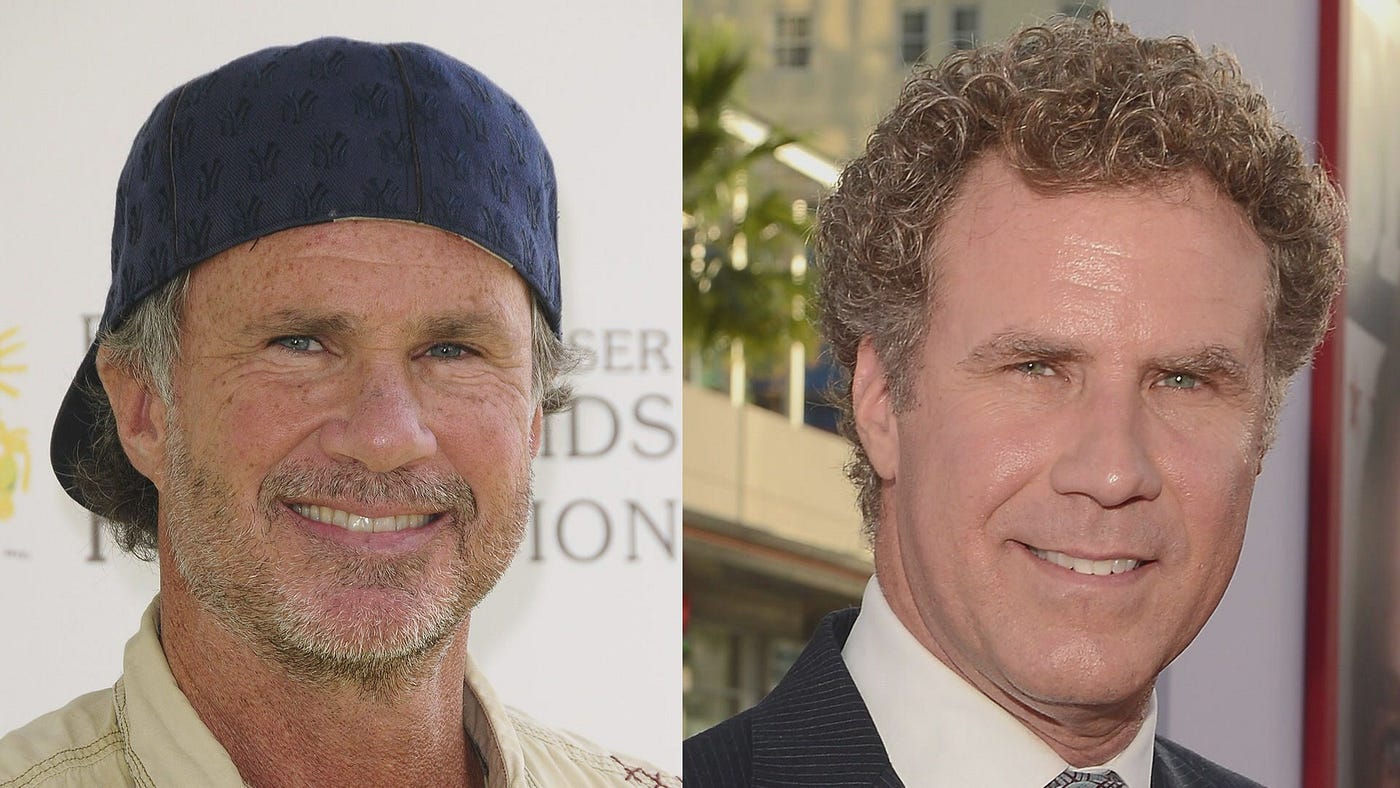
Let’s learn how modern face recognition works! But just recognizing your friends would be too easy. We can push this tech to the limit to solve a more challenging problem — telling Will Ferrell (famous actor) apart from Chad Smith (famous rock musician)!
One of these people is Will Farrell. The other is Chad Smith. I swear they are different people!
How to use Machine Learning on a Very Complicated Problem
But face recognition is really a series of several related problems:
First, look at a picture and find all the faces in it
Second, focus on each face and be able to understand that even if a face is turned in a weird direction or in bad lighting, it is still the same person.
Third, be able to pick out unique features of the face that you can use to tell it apart from other people— like how big the eyes are, how long the face is, etc.
Finally, compare the unique features of that face to all the people you already know to determine the person’s name.
As a human, your brain is wired to do all of this automatically and instantly. In fact, humans are too good at recognizing faces and end up seeing faces in everyday objects:
Computers are not capable of this kind of high-level generalization (at least not yet…), so we have to teach them how to do each step in this process separately.
We need to build a pipeline where we solve each step of face recognition separately and pass the result of the current step to the next step. In other words, we will chain together several machine learning algorithms:
How a basic pipeline for detecting faces might work
Face Recognition — Step by Step
Let’s tackle this problem one step at a time. For each step, we’ll learn about a different machine learning algorithm. I’m not going to explain every single algorithm completely to keep this from turning into a book, but you’ll learn the main ideas behind each one and you’ll learn how you can build your own facial recognition system in Python using OpenFace and dlib.
Step 1: Finding all the Faces
The first step in our pipeline is face detection. Obviously we need to locate the faces in a photograph before we can try to tell them apart!
If you’ve used any camera in the last 10 years, you’ve probably seen face detection in action:
Face detection is a great feature for cameras. When the camera can automatically pick out faces, it can make sure that all the faces are in focus before it takes the picture. But we’ll use it for a different purpose — finding the areas of the image we want to pass on to the next step in our pipeline.
Face detection went mainstream in the early 2000's when Paul Viola and Michael Jones invented a way to detect faces that was fast enough to run on cheap cameras. However, much more reliable solutions exist now. We’re going to use a method invented in 2005 called Histogram of Oriented Gradients — or just HOG for short.
To find faces in an image, we’ll start by making our image black and white because we don’t need color data to find faces:
Then we’ll look at every single pixel in our image one at a time. For every single pixel, we want to look at the pixels that directly surrounding it:
Our goal is to figure out how dark the current pixel is compared to the pixels directly surrounding it. Then we want to draw an arrow showing in which direction the image is getting darker:
Looking at just this one pixel and the pixels touching it, the image is getting darker towards the upper right.
If you repeat that process for every single pixel in the image, you end up with every pixel being replaced by an arrow. These arrows are called gradients and they show the flow from light to dark across the entire image:
This might seem like a random thing to do, but there’s a really good reason for replacing the pixels with gradients. If we analyze pixels directly, really dark images and really light images of the same person will have totally different pixel values. But by only considering the direction that brightness changes, both really dark images and really bright images will end up with the same exact representation. That makes the problem a lot easier to solve!
But saving the gradient for every single pixel gives us way too much detail. We end up missing the forest for the trees. It would be better if we could just see the basic flow of lightness/darkness at a higher level so we could see the basic pattern of the image.
To do this, we’ll break up the image into small squares of 16x16 pixels each. In each square, we’ll count up how many gradients point in each major direction (how many point up, point up-right, point right, etc…). Then we’ll replace that square in the image with the arrow directions that were the strongest.
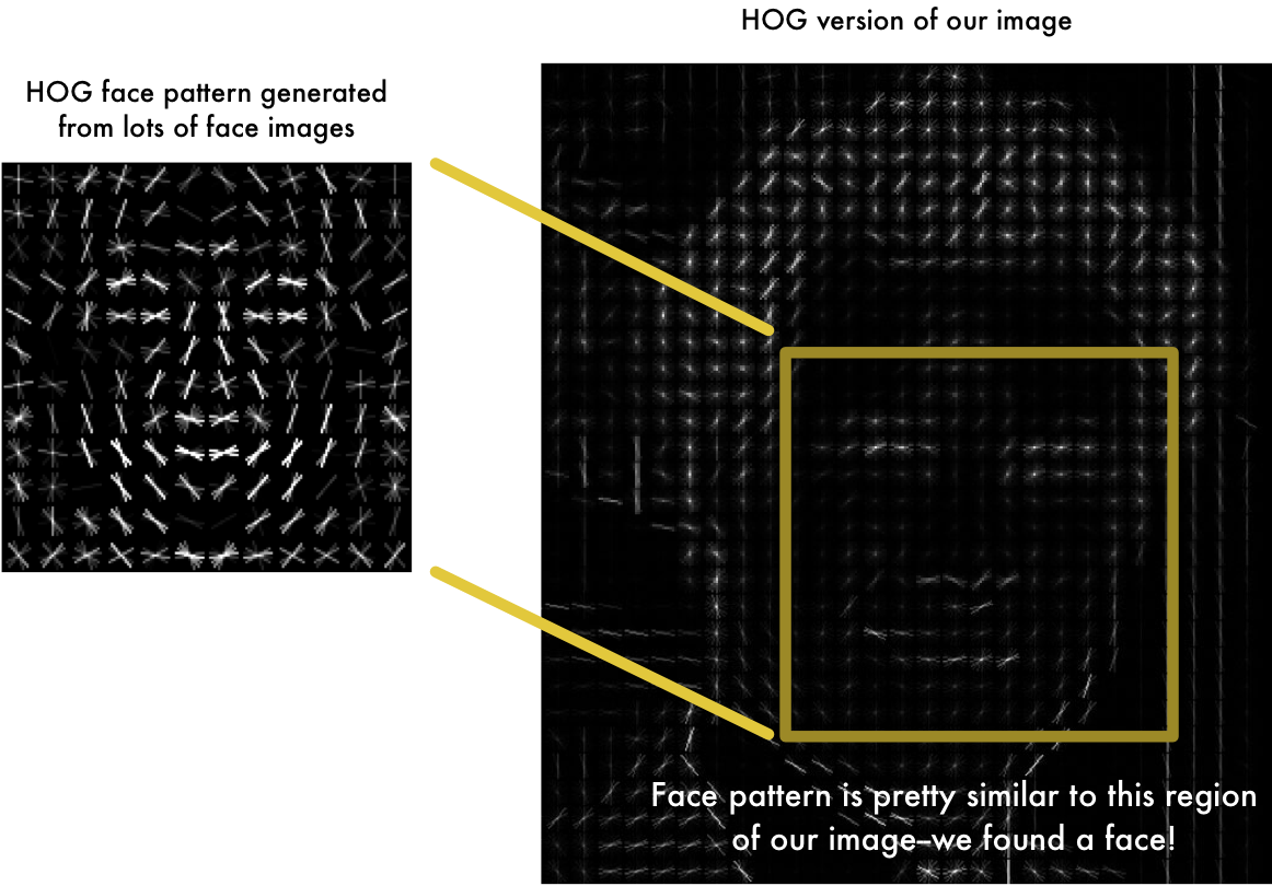
The end result is we turn the original image into a very simple representation that captures the basic structure of a face in a simple way:
The original image is turned into a HOG representation that captures the major features of the image regardless of image brightnesss.
To find faces in this HOG image, all we have to do is find the part of our image that looks the most similar to a known HOG pattern that was extracted from a bunch of other training faces:
Using this technique, we can now easily find faces in any image:
If you want to try this step out yourself using Python and dlib, here’s code showing how to generate and view HOG representations of images.
Step 2: Posing and Projecting Faces
Whew, we isolated the faces in our image. But now we have to deal with the problem that faces turned different directions look totally different to a computer:
Humans can easily recognize that both images are of Will Ferrell, but computers would see these pictures as two completely different people.
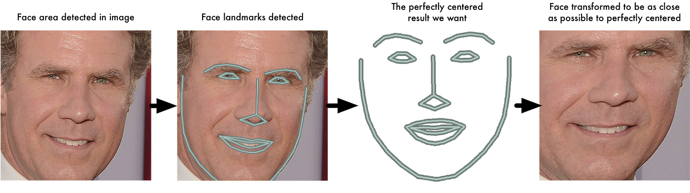
To account for this, we will try to warp each picture so that the eyes and lips are always in the sample place in the image. This will make it a lot easier for us to compare faces in the next steps.
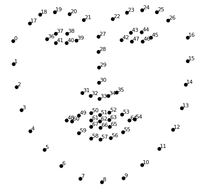
The basic idea is we will come up with 68 specific points (called landmarks) that exist on every face — the top of the chin, the outside edge of each eye, the inner edge of each eyebrow, etc. Then we will train a machine learning algorithm to be able to find these 68 specific points on any face:
The 68 landmarks we will locate on every face. This image was created by Brandon Amos of CMU who works on OpenFace.
Here’s the result of locating the 68 face landmarks on our test image:
PROTIP: You can also use this same technique to implement your own version of Snapchat’s real-time 3d face filters!
Now that we know were the eyes and mouth are, we’ll simply rotate, scale and shear the image so that the eyes and mouth are centered as best as possible. We won’t do any fancy 3d warps because that would introduce distortions into the image. We are only going to use basic image transformations like rotation and scale that preserve parallel lines (called affine transformations):
Now no matter how the face is turned, we are able to center the eyes and mouth are in roughly the same position in the image. This will make our next step a lot more accurate.
Now we are to the meat of the problem — actually telling faces apart. This is where things get really interesting!
The simplest approach to face recognition is to directly compare the unknown face we found in Step 2 with all the pictures we have of people that have already been tagged. When we find a previously tagged face that looks very similar to our unknown face, it must be the same person. Seems like a pretty good idea, right?
There’s actually a huge problem with that approach. A site like Facebook with billions of users and a trillion photos can’t possibly loop through every previous-tagged face to compare it to every newly uploaded picture. That would take way too long. They need to be able to recognize faces in milliseconds, not hours.
What we need is a way to extract a few basic measurements from each face. Then we could measure our unknown face the same way and find the known face with the closest measurements. For example, we might measure the size of each ear, the spacing between the eyes, the length of the nose, etc. If you’ve ever watched a bad crime show like CSI, you know what I am talking about:
Just like TV! So real! #science
The most reliable way to measure a face
Ok, so which measurements should we collect from each face to build our known face database? Ear size? Nose length? Eye color? Something else?
It turns out that the measurements that seem obvious to us humans (like eye color) don’t really make sense to a computer looking at individual pixels in an image. Researchers have discovered that the most accurate approach is to let the computer figure out the measurements to collect itself. Deep learning does a better job than humans at figuring out which parts of a face are important to measure.
The solution is to train a Deep Convolutional Neural Network (just like we did in Part 3). But instead of training the network to recognize pictures objects like we did last time, we are going to train it to generate 128 measurements for each face.
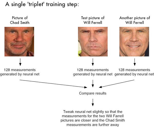
The training process works by looking at 3 face images at a time:
Load a training face image of a known person
Load another picture of the same known person
Load a picture of a totally different person
Then the algorithm looks at the measurements it is currently generating for each of those three images. It then tweaks the neural network slightly so that it makes sure the measurements it generates for #1 and #2 are slightly closer while making sure the measurements for #2 and #3 are slightly further apart:
After repeating this step millions of times for millions of images of thousands of different people, the neural network learns to reliably generate 128 measurements for each person. Any ten different pictures of the same person should give roughly the same measurements.
Machine learning people call the 128 measurements of each face an embedding. The idea of reducing complicated raw data like a picture into a list of computer-generated numbers comes up a lot in machine learning (especially in language translation). The exact approach for faces we are using was invented in 2015 by researchers at Google but many similar approaches exist.
Encoding our face image
This process of training a convolutional neural network to output face embeddings requires a lot of data and computer power. Even with an expensive NVidia Telsa video card, it takes about 24 hours of continuous training to get good accuracy.
But once the network has been trained, it can generate measurements for any face, even ones it has never seen before! So this step only needs to be done once. Lucky for us, the fine folks at OpenFace already did this and they published several trained networks which we can directly use. Thanks Brandon Amos and team!
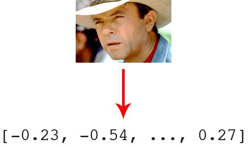
So all we need to do ourselves is run our face images through their pre-trained network to get the 128 measurements for each face. Here’s the measurements for our test image:
So what parts of the face are these 128 numbers measuring exactly? It turns out that we have no idea. It doesn’t really matter to us. All that we care is that the network generates nearly the same numbers when looking at two different pictures of the same person.
If you want to try this step yourself, OpenFace provides a lua script that will generate embeddings all images in a folder and write them to a csv file. You run it like this.
Step 4: Finding the person’s name from the encoding
This last step is actually the easiest step in the whole process. All we have to do is find the person in our database of known people who has the closest measurements to our test image.
You can do that by using any basic machine learning classification algorithm. No fancy deep learning tricks are needed. We’ll use a simple linear SVM classifier, but lots of classification algorithms could work.
All we need to do is train a classifier that can take in the measurements from a new test image and tells which known person is the closest match. Running this classifier takes milliseconds. The result of the classifier is the name of the person!
So let’s try out our system. First, I trained a classifier with the embeddings of about 20 pictures each of Will Ferrell, Chad Smith and Jimmy Falon:
It works! And look how well it works for faces in different poses — even sideways faces!
Running this Yourself
Let’s review the steps we followed:
Encode a picture using the HOG algorithm to create a simplified version of the image. Using this simplified image, find the part of the image that most looks like a generic HOG encoding of a face.
Figure out the pose of the face by finding the main landmarks in the face. Once we find those landmarks, use them to warp the image so that the eyes and mouth are centered.
Pass the centered face image through a neural network that knows how to measure features of the face. Save those 128 measurements.
Looking at all the faces we’ve measured in the past, see which person has the closest measurements to our face’s measurements. That’s our match!
Now that you know how this all works, here’s instructions from start-to-finish of how run this entire face recognition pipeline on your own computer:
UPDATE 4/9/2017:You can still follow the steps below to use OpenFace. However, I’ve released a new Python-based face recognition library called face_recognition that is much easier to install and use. So I’d recommend trying out face_recognition first instead of continuing below!
Note:For the following installs, ensure you are in a Python virtual environment if you’re using one. I highly recommend virtual environments for isolating your projects — it is a Python best practice. If you’ve followed my OpenCV install guides (and installed
virtualenv +
virtualenvwrapper ) then you can use the
workon
command prior to installing dlib and face_recognition.
Face recognition with OpenCV, Python, and deep learning
Inside this tutorial, you will learn how to perform facial recognition using OpenCV, Python, and deep learning.
We’ll start with a brief discussion of how deep learning-based facial recognition works, including the concept of “deep metric learning.”
From there, I will help you install the libraries you need to actually perform face recognition.
Finally, we’ll implement face recognition for both still images and video streams.
As we’ll discover, our face recognition implementation will be capable of running in real-time.
Understanding deep learning face recognition embeddings
So, how does deep learning + face recognition work?
The secret is a technique called deep metric learning.
If you have any prior experience with deep learning you know that we typically train a network to:
Accept a single input image
And output a classification/label for that image
However, deep metric learning is different.
Instead, of trying to output a single label (or even the coordinates/bounding box of objects in an image), we are instead outputting a real-valued feature vector.
For the dlib facial recognition network, the output feature vector is 128-d (i.e., a list of 128 real-valued numbers) that is used to quantify the face. Training the network is done using triplets:
Figure 1: Facial recognition via deep metric learning involves a “triplet training step.” The triplet consists of 3 unique face images — 2 of the 3 are the same person. The NN generates a 128-d vector for each of the 3 face images. For the 2 face images of the same person, we tweak the neural network weights to make the vector closer via distance metric. Image credit:Adam Geitgey’s “Machine Learning is Fun” blog
Here we provide three images to the network:
Two of these images are example faces of the same person.
The third image is a random face from our dataset and is not the same person as the other two images.
As an example, let’s again consider Figure 1 where we provided three images: one of Chad Smith and two of Will Ferrell.
Our network quantifies the faces, constructing the 128-d embedding (quantification) for each.
From there, the general idea is that we’ll tweak the weights of our neural network so that the 128-d measurements of the two Will Ferrel will be closer to each other and farther from the measurements for Chad Smith.
Our network architecture for face recognition is based on ResNet-34 from the Deep Residual Learning for Image Recognition paper by He et al., but with fewer layers and the number of filters reduced by half.
The network itself was trained by Davis King on a dataset of ≈3 million images. On the Labeled Faces in the Wild (LFW) dataset the network compares to other state-of-the-art methods, reaching 99.38% accuracy.
Both Davis King (the creator of dlib) and Adam Geitgey (the author of the face_recognition module we’ll be using shortly) have written detailed articles on how deep learning-based facial recognition works:
The dlib library, maintained by Davis King, contains our implementation of “deep metric learning” which is used to construct our face embeddings used for the actual recognition process.
The
face_recognition
library, created by Adam Geitgey, wraps around dlib’s facial recognition functionality, making it easier to work with.
I assume that you have OpenCV installed on your system. If not, no worries — just visit my OpenCV install tutorials page and follow the guide appropriate for your system.
From there, let’s install
dlib
and the
face_recognition
packages.
Note:For the following installs, ensure you are in a Python virtual environment if you’re using one. I highly recommend virtual environments for isolating your projects — it is a Python best practice. If you’ve followed my OpenCV install guides (and installed
Face recognition with OpenCV, Python, and deep learning
$ workon <your env name here> # optional
$ pip install imutils
Our face recognition dataset
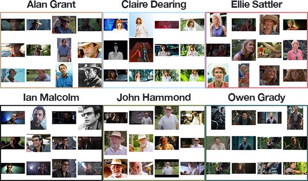
Figure 2: An example face recognition dataset was created programmatically with Python and the Bing Image Search API. Shown are six of the characters from the Jurassic Park movie series.
Since Jurassic Park (1993) is my favorite movie of all time, and in honor of Jurassic World: Fallen Kingdom (2018) being released this Friday in the U.S., we are going to apply face recognition to a sample of the characters in the films:
Face recognition with OpenCV, Python, and deep learning
$ tree --filelimit 10 --dirsfirst
.
├── dataset
│ ├── alan_grant [22 entries]
│ ├── claire_dearing [53 entries]
│ ├── ellie_sattler [31 entries]
│ ├── ian_malcolm [41 entries]
│ ├── john_hammond [36 entries]
│ └── owen_grady [35 entries]
├── examples
│ ├── example_01.png
│ ├── example_02.png
│ └── example_03.png
├── output
│ └── lunch_scene_output.avi
├── videos
│ └── lunch_scene.mp4
├── search_bing_api.py
├── encode_faces.py
├── recognize_faces_image.py
├── recognize_faces_video.py
├── recognize_faces_video_file.py
└── encodings.pickle
10 directories, 11 files
Our project has 4 top-level directories:
dataset/
: Contains face images for six characters organized into subdirectories based on their respective names.
examples/
: Has three face images for testing that are not in the dataset.
output/
: This is where you can store your processed face recognition videos. I’m leaving one of mine in the folder — the classic “lunch scene” from the original Jurassic Park movie.
videos/
: Input videos should be stored in this folder. This folder also contains the “lunch scene” video but it hasn’t undergone our face recognition system yet.
We also have 6 files in the root directory:
search_bing_api.py
: Step 1 is to build a dataset (I’ve already done this for you). To learn how to use the Bing API to build a dataset with my script, just see this blog post.
encode_faces.py
: Encodings (128-d vectors) for faces are built with this script.
recognize_faces_image.py
: Recognize faces in a single image (based on encodings from your dataset).
recognize_faces_video.py
: Recognize faces in a live video stream from your webcam and output a video.
recognize_faces_video_file.py
: Recognize faces in a video file residing on disk and output the processed video to disk. I won’t be discussing this file today as the bones are from the same skeleton as the video stream file.
encodings.pickle
: Facial recognitions encodings are generated from your dataset via
encode_faces.py
and then serialized to disk.
After a dataset of images is created (with
search_bing_api.py
), we’ll run
encode_faces.py
to build the embeddings.
From there, we’ll run the recognize scripts to actually recognize the faces.
Encoding the faces using OpenCV and deep learning
Figure 3: Facial recognition via deep learning and Python using the face_recognition module method generates a 128-d real-valued number feature vector per face.
Before we can recognize faces in images and videos, we first need to quantify the faces in our training set. Keep in mind that we are not actually training a network here — the network has already been trained to create 128-d embeddings on a dataset of
~3
million images.
We certainly could train a network from scratch or even fine-tune the weights of an existing model but that is more than likely overkill for many projects. Furthermore, you would need a lot of images to train the network from scratch.
Instead, it’s easier to use the pre-trained network and then use it to construct 128-d embeddings for each of the 218 faces in our dataset.
Then, during classification, we can use a simple k-NN model + votes to make the final face classification. Other traditional machine learning models can be used here as well.
To construct our face embeddings open up
encode_faces.py
from the “Downloads” associated with this blog post:
help="face detection model to use: either `hog` or `cnn`")
args = vars(ap.parse_args())
If you’re new to PyImageSearch, let me direct your attention to the above code block which will become familiar to you as you read more of my blog posts. We’re using
argparse
to parse command line arguments. When you run a Python program in your command line, you can provide additional information to the script without leaving your terminal. Lines 10-17 do not need to be modified as they parse input coming from the terminal. Check out my blog post about command line arguments if these lines look unfamiliar.
Let’s list out the argument flags and discuss them:
--dataset
: The path to our dataset (we created a dataset with
# add each encoding + name to our set of known names and
# encodings
knownEncodings.append(encoding)
knownNames.append(name)
This is the fun part of the script!
For each iteration of the loop, we’re going to detect a face (or possibly multiple faces and assume that it is the same person in multiple locations of the image — this assumption may or may not hold true in your own images so be careful here).
For example, let’s say that
rgb
contains a picture (or pictures) of Ellie Sattler’s face.
Lines 41 and 42 actually find/localize the faces of her resulting in a list of face
boxes
. We pass two parameters to the
face_recognition.face_locations
method:
rgb
: Our RGB image.
model
: Either
cnn
or
hog
(this value is contained within our command line arguments dictionary associated with the
"detection_method"
key). The CNN method is more accurate but slower. HOG is faster but less accurate.
Then, we’re going to turn the bounding
boxes
of Ellie Sattler’s face into a list of 128 numbers on Line 45. This is known as encoding the face into a vector and the
face_recognition.face_encodings
method handles it for us.
From there we just need to append the Ellie Sattler
encoding
and
name
to the appropriate list (
knownEncodings
and
knownNames
).
We’ll continue to do this for all 218 images in the dataset.
What would be the point of encoding the images unless we could use the
-rw-r--r--@ 1 adrian staff 234K May 2913:03 encodings.pickle
As you can see from our output, we now have a file named
encodings.pickle
— this file contains the 128-d face embeddings for each face in our dataset.
On my Titan X GPU, processing the entire dataset took a little over a minute, but if you’re using a CPU, be prepared to wait awhile for this script complete!
On my Macbook Pro (no GPU), encoding 218 images required 21min 20sec.
You should expect much faster speeds if you have a GPU and compiled dlib with GPU support.
Recognizing faces in images
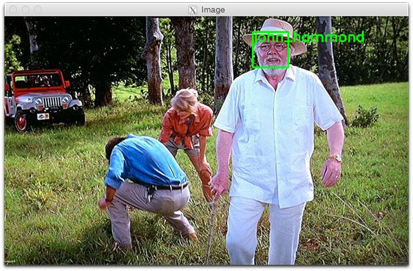
Figure 4: John Hammond’s face is recognized using Adam Geitgey’s deep learning face_recognition Python module.
Now that we have created our 128-d face embeddings for each image in our dataset, we are now ready to recognize faces in image using OpenCV, Python, and deep learning.
Open up
recognize_faces_image.py
and insert the following code (or better yet, grab the files and image data associated with this blog post from the “Downloads” section found at the bottom of this post, and follow along):
On Line 37, we begin to loop over the face encodings computed from our input image.
Then the facial recognition magic happens!
We attempt to match each face in the input image (
encoding
) to our known encodings dataset (held in
data["encodings"]
) using
face_recognition.compare_faces
(Lines 40 and 41).
This function returns a list of
True
/
False
values, one for each image in our dataset. For our Jurassic Park example, there are 218 images in the dataset and therefore the returned list will have 218 boolean values.
Internally, the
compare_faces
function is computing the Euclidean distance between the candidate embedding and all faces in our dataset:
If the distance is below some tolerance (the smaller the tolerance, the more strict our facial recognition system will be) then we return
True
, indicating the faces match.
Otherwise, if the distance is above the tolerance threshold we return
On Line 67, we begin looping over the detected face bounding
boxes
and predicted
names
. To create an iterable object so we can easily loop through the values, we call
zip(boxes, names)
resulting in tuples that we can extract the box coordinates and name from.
We use the box coordinates to draw a green rectangle on Line 69.
We also use the coordinates to calculate where we should draw the text for the person’s name (Line 70) followed by actually placing the name text on the image (Lines 71 and 72). If the face bounding box is at the very top of the image, we need to move the text below the top of the box (handled on Line 70), otherwise, the text would be cut off.
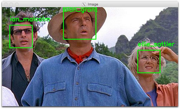
We then proceed to display the image until a key is pressed (Lines 75 and 76).
How should you run the facial recognition Python script?
Using your terminal, first ensure you’re in your respective Python correct virtual environment with the
workon
command (if you are using a virtual environment, of course).
Then run the script while providing the two command line arguments at a minimum. If you choose to use the HoG method, be sure to pass
--detection-method hog
as well (otherwise it will default to the deep learning detector).
Let’s go for it!
To recognize a face using OpenCV and Python open up your terminal and execute our script:
Figure 6: Face recognition with OpenCV and Python.
Recognizing faces in video
Figure 7: Face recognition for videos with OpenCV and Python.
Now that we have applied face recognition to images let’s also apply face recognition to videos (in real-time) as well.
Important Performance Note:The CNN face recognizer should only be used in real-time if you are working with a GPU (you can use it with a CPU, but expect less than 0.5 FPS which makes for a choppy video). Alternatively (you are using a CPU), you should use the HoG method (or even OpenCV Haar cascades covered in a future blog post) and expect adequate speeds.
The following script draws many parallels from the previous
recognize_faces_image.py
script. Therefore I’ll be breezing past what we’ve already covered and just review the video components so that you understand what is going on.
Face recognition with OpenCV, Python, and deep learning
# load the known faces and embeddings
print("[INFO] loading encodings...")
data = pickle.loads(open(args["encodings"], "rb").read())
# initialize the video stream and pointer to output video file, then
# allow the camera sensor to warm up
print("[INFO] starting video stream...")
vs = VideoStream(src=0).start()
writer = None
time.sleep(2.0)
To access our camera we’re using the
VideoStream
class from imutils. Line 29 starts the stream. If you have multiple cameras on your system (such as a built-in webcam and an external USB cam), you can change the
src=0
to
src=1
and so forth.
We’ll be optionally writing processed video frames to disk later, so we initialize
writer
to
None
(Line 30). Sleeping for 2 complete seconds allows our camera to warm up (Line 31).
Our loop begins on Line 34 and the first step we take is to grab a
frame
from the video stream (Line 36).
The remaining Lines 40-50 in the above code block are nearly identical to the lines in the previous script with the exception being that this is a video frame and not a static image. Essentially we read the
# loop over the matched indexes and maintain a count for
# each recognized face face
for i in matchedIdxs:
name = data["names"][i]
counts[name] = counts.get(name, 0) + 1
# determine the recognized face with the largest number
# of votes (note: in the event of an unlikely tie Python
# will select first entry in the dictionary)
name = max(counts, key=counts.get)
# update the list of names
names.append(name)
In this code block, we loop over each of the
encodings
and attempt to match the face. If there are matches found, we count the votes for each name in the dataset. We then extract the highest vote count and that is the name associated with the face. These lines are identical to the previous script we reviewed, so let’s move on.
In this next block, we loop over the recognized faces and proceed to draw a box around the face and the display name of the person above the face:
Below you can find an output example video that I recorded demonstrating the face recognition system in action:
Face recognition in video files
As I mentioned in our “Face recognition project structure” section, there’s an additional script included in the “Downloads” for this blog post —
recognize_faces_video_file.py
.
This file is essentially the same as the one we just reviewed for the webcam except it will take an input video file and generate an output video file if you’d like.
I applied our face recognition code to the popular “lunch scene” from the original Jurassic Park movie where the cast is sitting around a table sharing their concerns with the park:
Note:Recall that our model was trained on four members of the original cast: Alan Grant, Ellie Sattler, Ian Malcolm, and John Hammond. The model was not trained on Donald Gennaro (the lawyer) which is why his face is labeled as “Unknown”. This behavior was by design (not an accident) to show that our face recognition system can recognize faces it was trained on while leaving faces it cannot recognize as “Unknown”.
And in the following video I have put together a “highlight reel” of Jurassic Park and Jurassic World clips, mainly from the trailers:
As we can see, we can see, our face recognition and OpenCV code works quite well!